Image Analysis - Histogram Analysis

We often want to generate images that are of appropriate quality for a task at hand. It is therefore possible to gain a general idea about an images quality through it’s distribution of gray scale values.

• This distribution is the Gray Level Histogram (GLH)

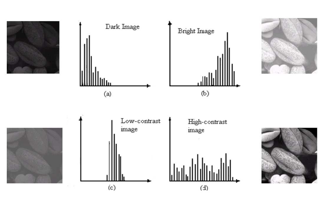
An image histogram, shows us the distribution of pixel intensity values across the available gray scale. Often revealing important features about an image.

We are able to guess how an image may appear simply by looking at its histogram:

Contrast Stretching

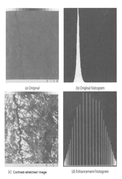
This is a technique that attempts to improve an image simply by stretching out the possible range of intensity values it contains to make full use of possible values.

This transformation would improve the contrast of an image, and make details easier to visualise.

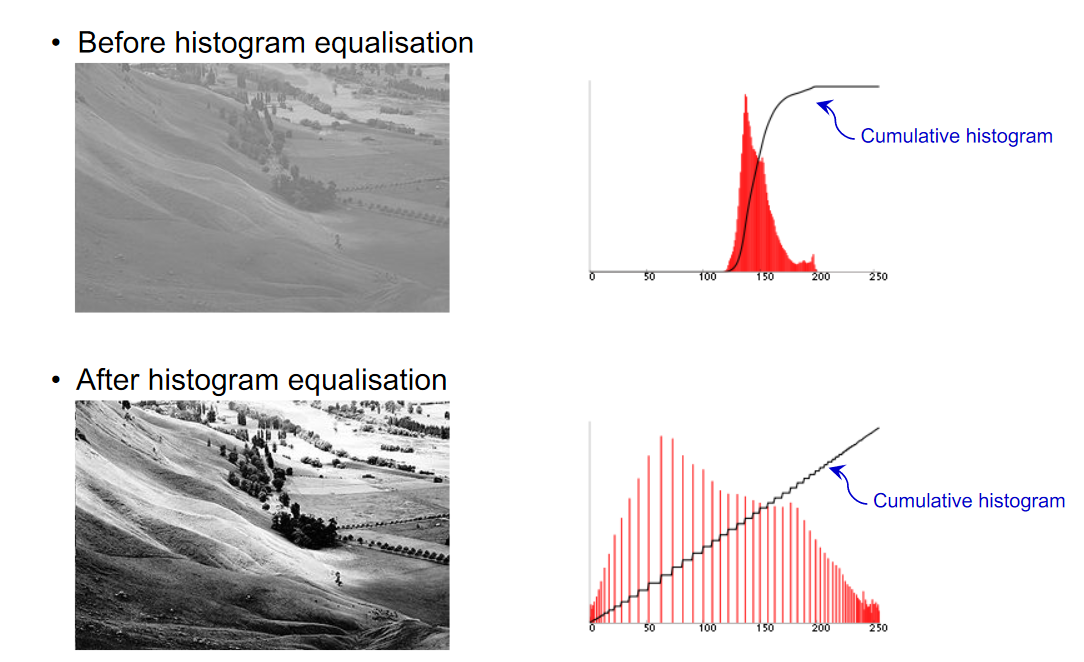
Transformation function: Histogram equalisation.

Histogram Equalisation is used as the transformation function for contrast stretching.

When an image contains regions that are significantly lighter or darker, then those regions would not be enhanced, preserving detail in the areas where it counts.

Python Code example:

import matplotlib.pyplot as plt
import numpy as np

X = np.array([
    [6, 3, 6, 5, 3, 3],
    [3, 6, 4, 6, 4, 5],
    [2, 3, 3, 2, 2, 5],
    [4, 3, 4, 6, 4, 6],
    [5, 4, 4, 4, 4, 6],
    [4, 4, 6, 6, 4, 6],
])  # sample 2D array
plt.imshow(X, cmap="gray", vmin=0, vmax=8)
plt.show()

X = np.array([
    [7, 2, 7, 5, 2, 2],
    [2, 7, 4, 7, 4, 5],
    [1, 2, 2, 1, 1, 5],
    [4, 2, 4, 7, 4, 7],
    [5, 4, 4, 4, 4, 7],
    [4, 4, 7, 7, 4, 7],
])  # sample 2D array
plt.imshow(X, cmap="gray", vmin=0, vmax=8)
plt.show()

figure_6 = {
    "0": 0,
    "1": 0,
    "2": 3,
    "3": 7,
    "4": 12,
    "5": 4,
    "6": 10,
}


def cumulative_freq_figure(figure=figure_6):
    cum_figure = {}
    c = 0
    for (index, value) in figure.items():
        c += value
        cum_figure[index] = c

    return cum_figure


def apply_histogram(figure, max_g=7, n=6, m=3):

    equalised_figure = {}
    for g in range(0, max_g):
        first_part = ((2 ** m) - 1) / (n ** 2)
        second_part = figure[str(g)]

        result = first_part * second_part

        print(str(g) + ': ' + str(result) + ' rounded to -> ' + str(round(result)))

        equalised_figure[str(g)] = round(result)

    print(equalised_figure)

    return equalised_figure
    # (figure[str(g)])


def app():
    print('RESULTS')
    print('CUMULATIVE FIGURE')
    cum_figure = cumulative_freq_figure(figure_6)

    print(cum_figure)

    print('EQUALISED')
    print(apply_histogram(cum_figure))


if __name__ == '__main__':
    app()

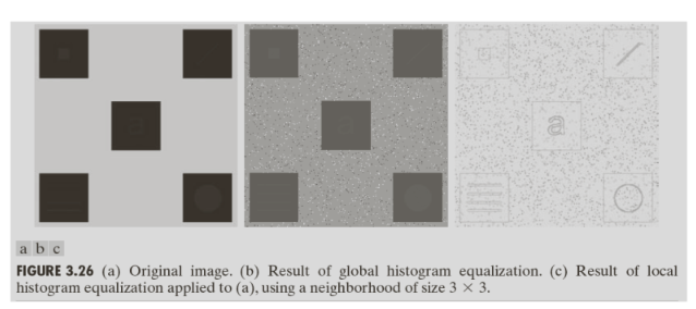
Local / Adaptive Histogram equalisation

Transformation of each pixel with a transformation function derived from its neighborhood region. The size of the region has an impact on the output produced.

Summary

• Gray level histograms can give us an indication about the quality of an image, even though it is one of simplest approaches to this.
• Images can even be enhanced to improve appearance for human viewing.
• Histogram equalisation can be achieved through point operation or neighborhood operations.